Images
Ambient Occlusion
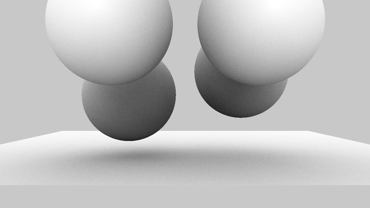
Ambient Occlusion is the first project I made after taking up ray tracing again. In standard basic ray tracing, shadows are normally very sharp. The shadow in the traditional ray tracing algorithm is calculated by testing if there is a free line of sight between a light-source point and point in the scene being examined.
Ambient Occlusion goes another way. Instead of having a single point of light in the scene the entire sphere around the scene is considered a light source. A bunch of rays are emitted from the point in the scene being examined. The rays are emitted in random directions within a hemisphere. The number of rays emitted are called N. The number of rays not hitting any objects are called m.
The light intensity is now calculated as the ratio m/N.
If 100 rays are emitted and 10 of them hits other objects, then the light intensity would be 0.9.
The drawback of this algorithm is the number of rays that would have to be emitted from every point in the scene. Too few rays and the output image will look very noisy like an underexposed photography. Casting more rays like 1000 or 4000 rays from every point in the scene will give rendering times in hours or even days.
The result however is impressive. The image below took about an hour to compute. But the shadows looks very soft and realistic. Something that is normally very hard to obtain in a raytracer.
Notice the noise seen in the bigger version of the image.

Click on image to enlarge
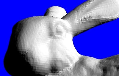
Stanford Bunny Model - Flat Shading
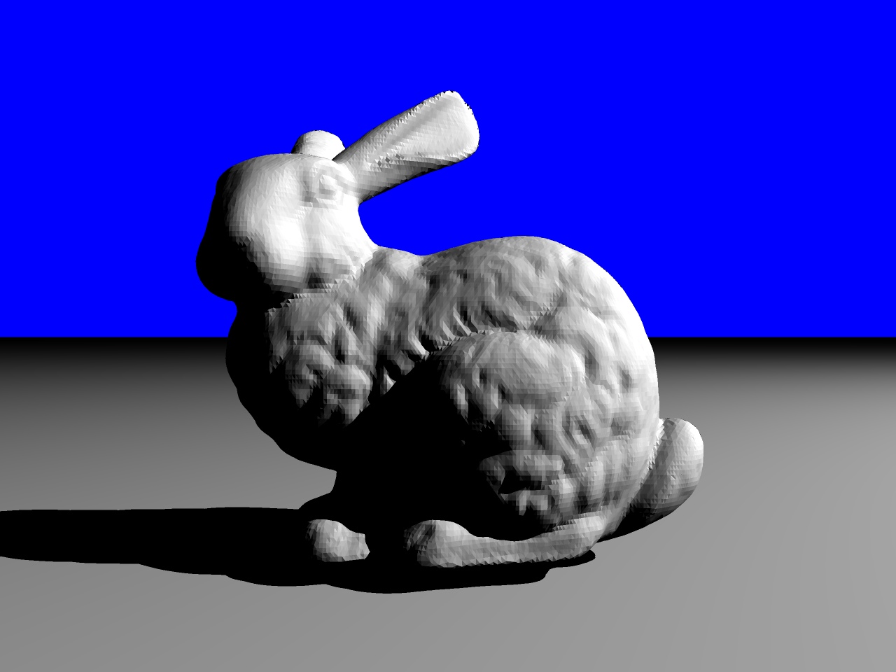
The model I used for this image is the Stanford Bunny - a 3d model often used to benchmark ray tracing algorithms. The model that I found on the homepage of "The Stanford 3D Scanning Repository" consists of vertices and faces (triangles). As seen in the image the triangles are very much visible. This is due to the flat shading model I used in my raytracer. Since I only have triangles in the model file, I calculate the normal for each triangle as a normal perpendicular to the surface. If you want a surface that looks smooth this is not the way to go. The number of triangles needed to give a smooth look is tremendous. This is why I later started to interpolate the normals as seen below.
Click on image to enlarge
Stanford Bunny Model - Interpolated Normals
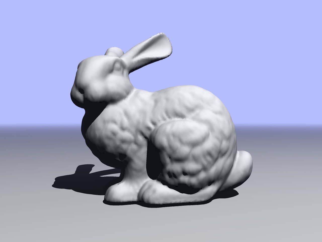
In this image I computed a normal for each vertex. When hitting a point inside a triangle, I computed a secondary normal as a sort of weighted average between the 3 normals on each of the triangles 3 vertices. The result is very smooth. Even for 3D models with very few triangles, the models look smooth. As the triangle count goes down however, the outline of the model gets more and more jaggy.

Click on image to enlarge
Cow Model - Binary Space Partition
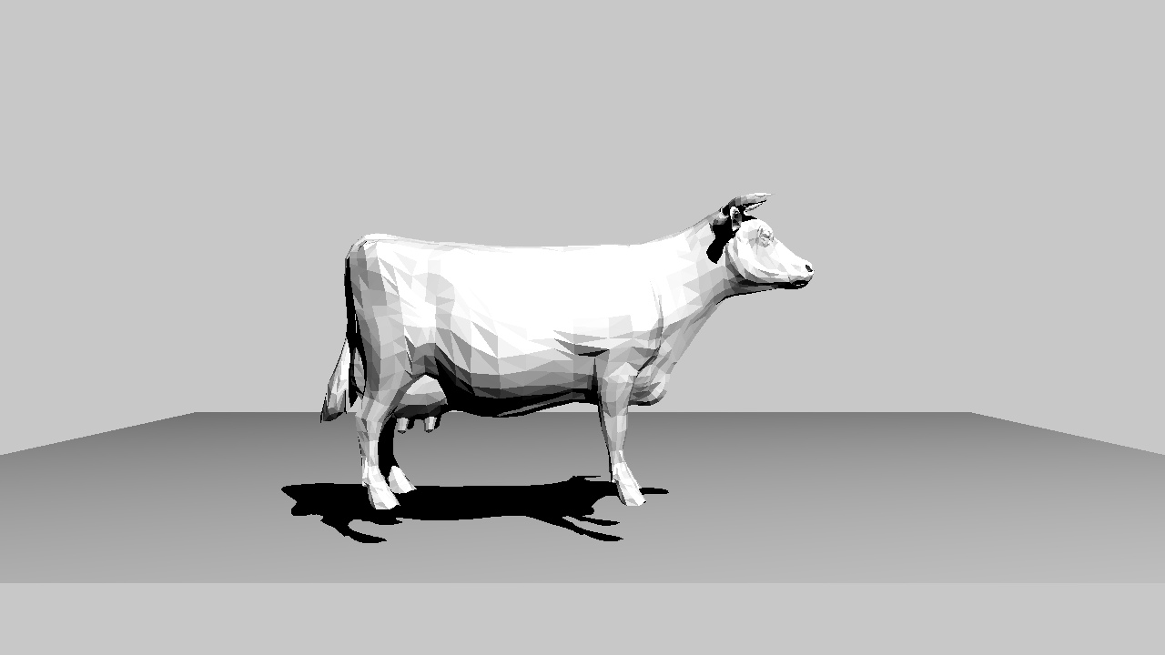
The bunny model consists of 69451 triangles and takes a lot of time to render. This is why I started on Binary Space Partitioning to speed up render times. For testing the algorithm I used a simpler model of a cow, where it was easier to see if I got it right or not and I had less data to debug through.
For each model I compute the minimum and maximum coordinates and fit a bounding box around the model. If a ray does not hit the bounding box of a model I go on to the next model, if the ray does hit the bounding box I examine the model further. I have divided the cow model into two by cutting it by a plane in the center of the x axis of the model. All triangles on one side the plane goes into a child bounding box, and all triangles on the other side goes to another child bounding box. If a triangle intersects the plane I put the triangle in both of the children bounding boxes. Now by recursively dividing each child bounding boxes a number of times I end up with hundreds of smaller bounding boxes.
The speed gain comes in that previously I had to test all triangles against each ray of each pixel in the image. A cow model of 5000 triangles and a image of 1280x960 pixels gave 6,144,000,000 intersection tests. With the Binary Space Partitioning the number of tests comes down to something like 2 or 3 million ray tests - a speed gain of a factor 1000 or more.

Click on image to enlarge
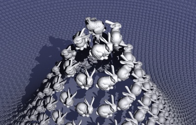
Stanford Bunny Model - Instancing
With the render time down to a few seconds I could move on to next step - throwing in hundreds or thousands of models. To produce the image below which consists of 909,391,394 triangles and 13092 bunnies a few more optimizations had to be made though.
For one, my ray-boundingbox test appeared to be a bottleneck. I optimized the intersection by thinking in Plucker coordinates in which the intersection is made by testing the ray against the silhouette of the box instead of the planes that the box consists of. With this single optimization I gained a speedup of 4.3 times in the entire rendering.
Next bottleneck was memory. The memory to contain the scene in the picture is counted in tens of gigabytes. Since all the bunnies look the same, I decided to implement instancing in which the bunny is stored only once. All the bunnies in the scene therefore only consists of a transformation matrix and a reference to the actual 3D model. The optimization sounds obvious but has a drawback. I can no longer use a single BSP tree for the entire scene.
Third optimization therefore was to make another BSP tree for all the instances of models in the scene. This gave a speed gain of a factor 17 and made it possible to render the 909,391,394 triangle scene below - my personal record so far.
Pretty strange image though :)
Click on image to enlarge
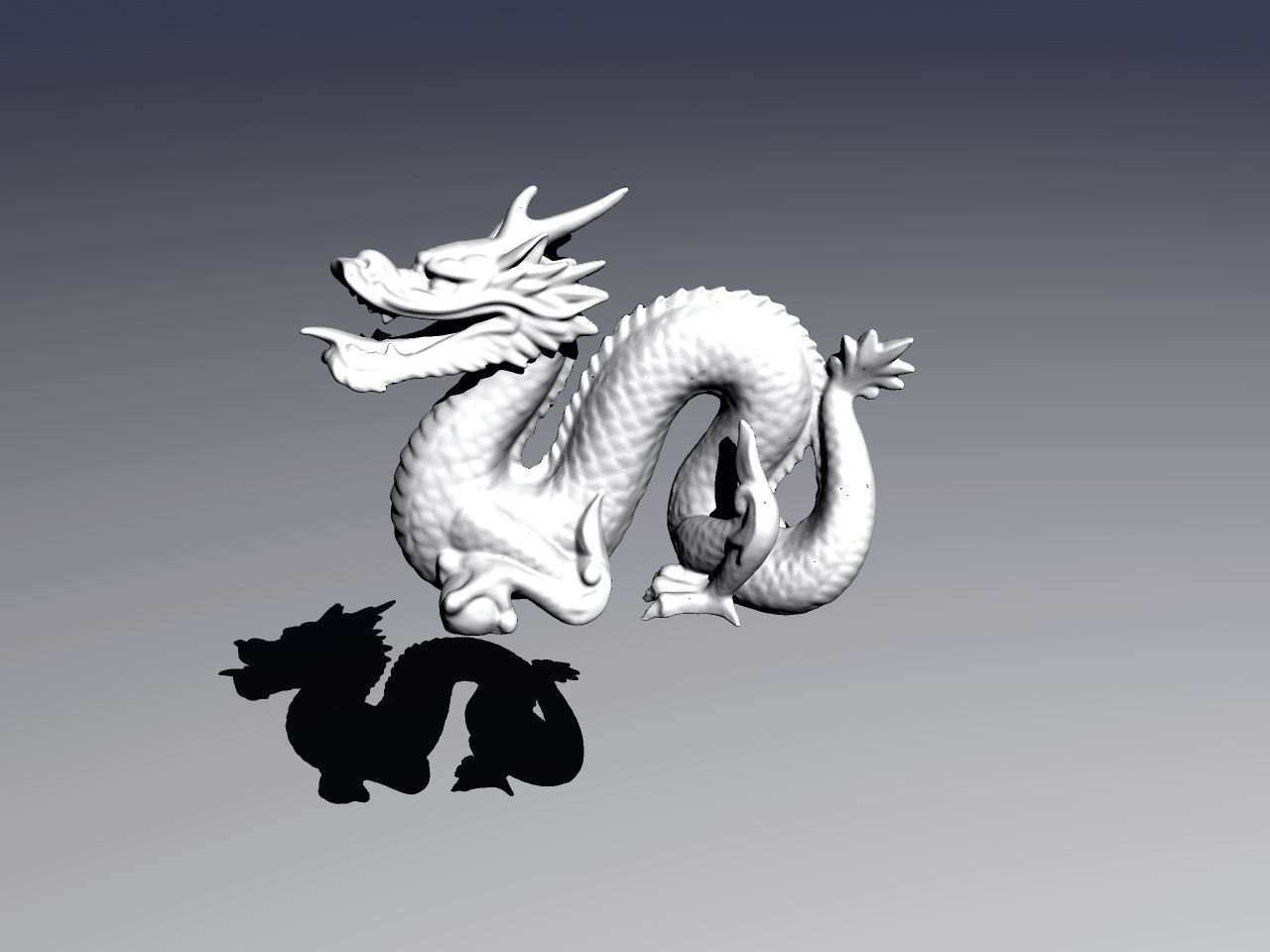
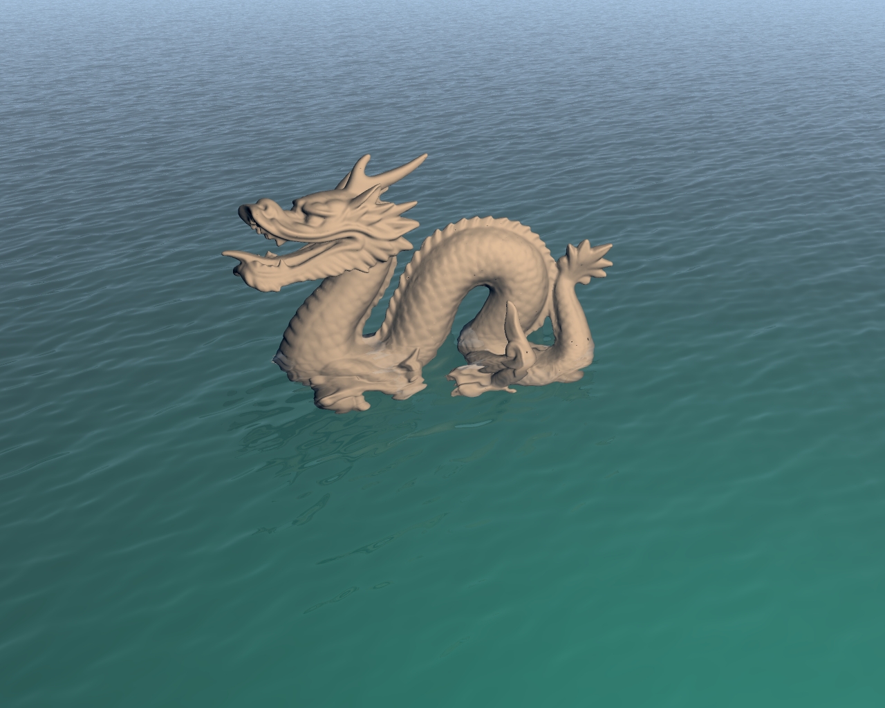
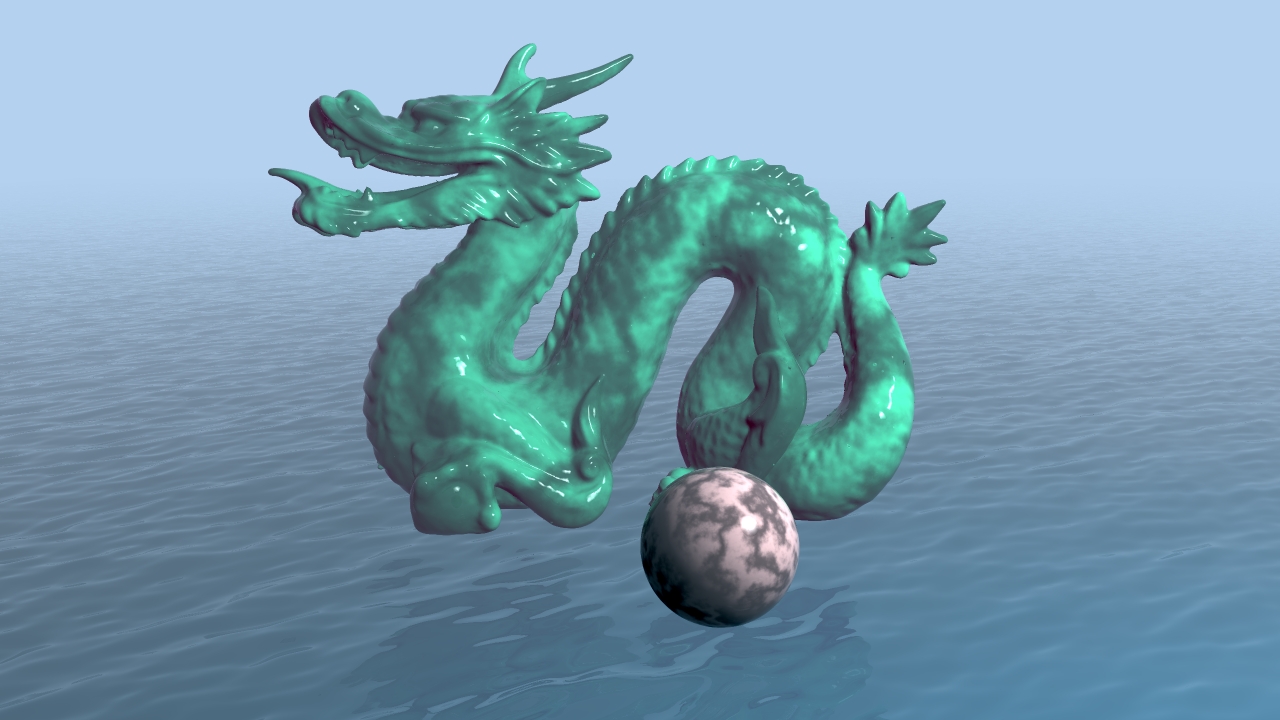
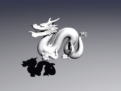
Chineese Dragon
This model contains 871414 triangles and forced me to rewrite my .ply model file reader a bit. The model comes without normal vectors and computing interpolated normals made my reader grind to a halt. Now rewritten I can render this model, which although it contains more than ten times as many triangles only takes twice as long to render.
Previously I stored the models as a C header file, which I included in my render source code. But the dragon caused the compiler preprocessor to choke, so I also implemented a simple binary file format, which also means that I dont have to recompile for every new model I want to ray trace.
Click on image to enlarge
Glass and Water
When developing the reflections and refractions I started testing the algorithms on flat planes and spheres. The results came out pretty boring, so I made a nicer geometric model of water waves. The water model was made by Fourier transforming a 2D spectrum of the distribution of waves in a typically deep water ocean. This way the waves tiles nice too, so I later can make larger oceans by instancing each wave tile. In this picture I use only one wave tile of about 25 meters on each side.
To make the surface look like water I found some formulas from my old Optics Class describing the fresnel terms. The fresnel term determines how much of the light is reflected and how much is transmitted through the surface. The term depends on the angle of incidence.
Next step will be to implement internal reflections as well, so I can ray trace underwater scenes.

Click on image to enlarge
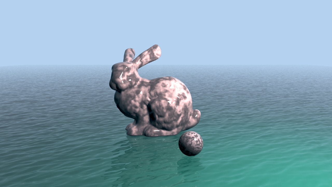
Internal Reflections
Internal reflections turned out to be much harder than external reflections. Also I seem to have some problems with the rendering along the edges of the complex bunny model. I could be due to the maximum recursions that I allow, but I also suspect the interpolated normals to give some problems. More to come!

Click on image to enlarge
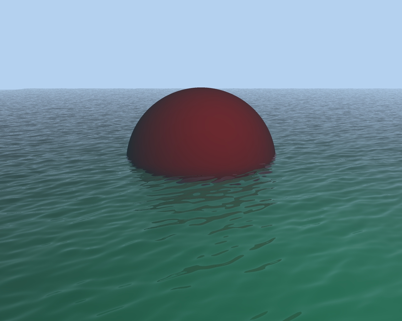
Ocean Model
The ocean is made from a model that is 25 times 25 meters across. The model is instanced 49 times in a 7 times 7 grid. By adding a little fog I disguise the abrupt stop of the ocean in the horizon.

Click on image to enlarge
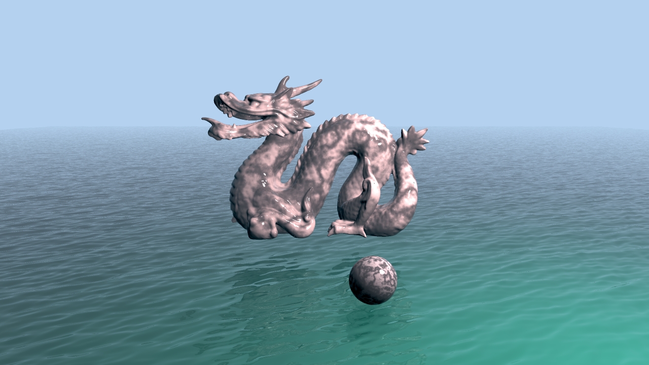
Bug fixing
A bug in my triangle sorting caused some triangles to be missing. But since the triangle are so small, the bug shows up as missing pixels. This is fixed now, and for fun I rendered the chineese dragon instead of the Stanford bunny. The dragon model has some small holes in the surface. This is from the model and not the rendering.

Click on image to enlarge
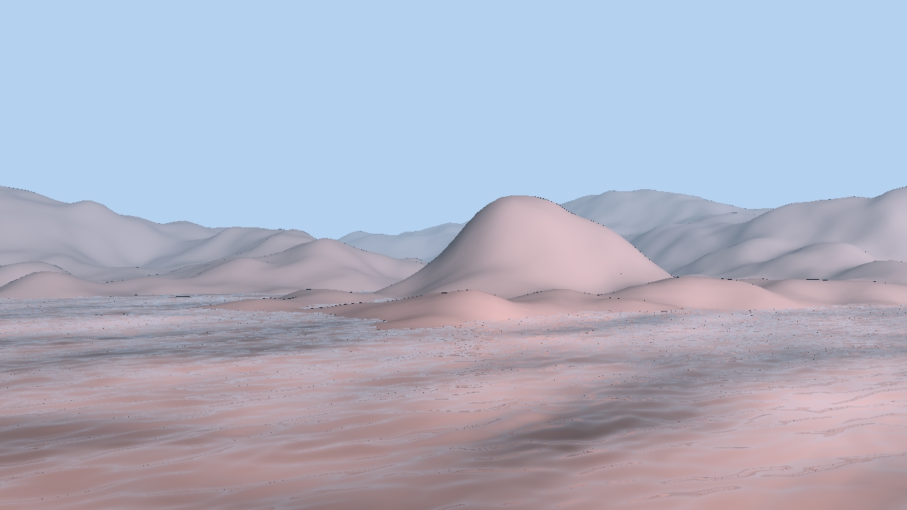
Landscapes
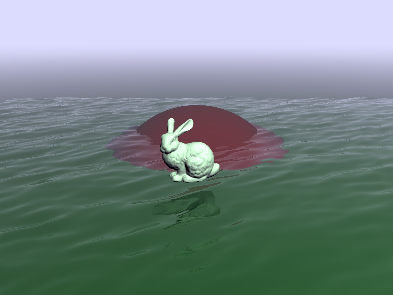
A first attempt to make landscapes. I made a simple converter from a image file into a 3D model and simply used that model as an object in my raytracer. The terrain was made in Photoshop by drawing and adding some noise and then blurring it again to avoid too sharp edges.
My raytracer lacks quite a lot features yet. I could need some texture mapping, bump mapping a better lightmodel for atmospheric phenomena.
The ocean looks pink because it is entirely transparent and the ocean floor is pink.

Click on image to enlarge
Marble - Procedural Texture
First attempt to make textures. The texture is a procedural texture based on Perlin noise. I haven't really implemented Phong highlights yet in the shader, so the white spots are actually real reflections of a big white sphere placed behind the light-source.

Click on image to enlarge

Click on image to enlarge
Click on image to enlarge
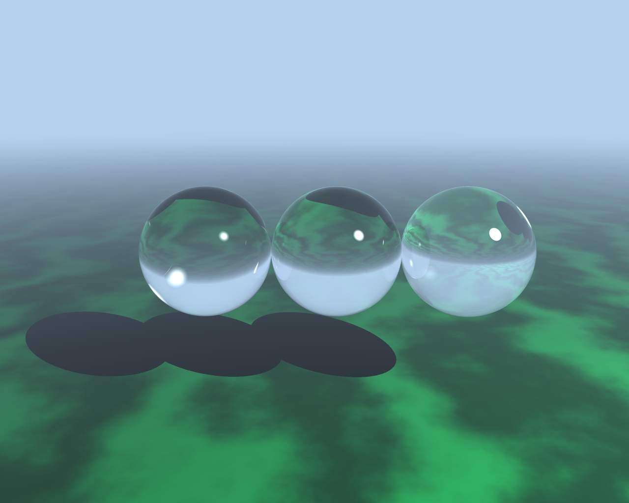
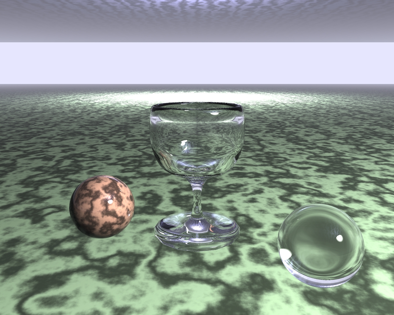
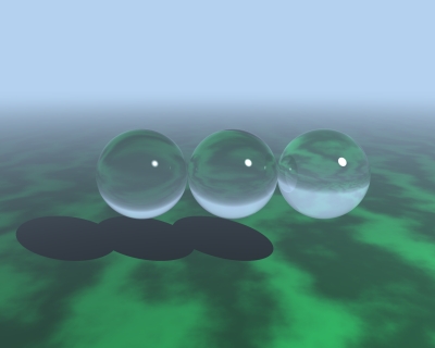
Refraction - Water, Glass and Diamonds
The glass material is made a bit more flexible. Earlier the index of refraction was hardcoded to 1.33 which corresponds to water. Now I have support for whatever desired index of refraction. The index of refraction contributes to both how much the rays are bent, but also how much light is reflected and refracted. The latter depends on the angle of incidence and is the factor that really makes water look like water.
The test image below show three spheres from left to right: Water, Glass and Diamond.
Click on image to enlarge

Click on image to enlarge
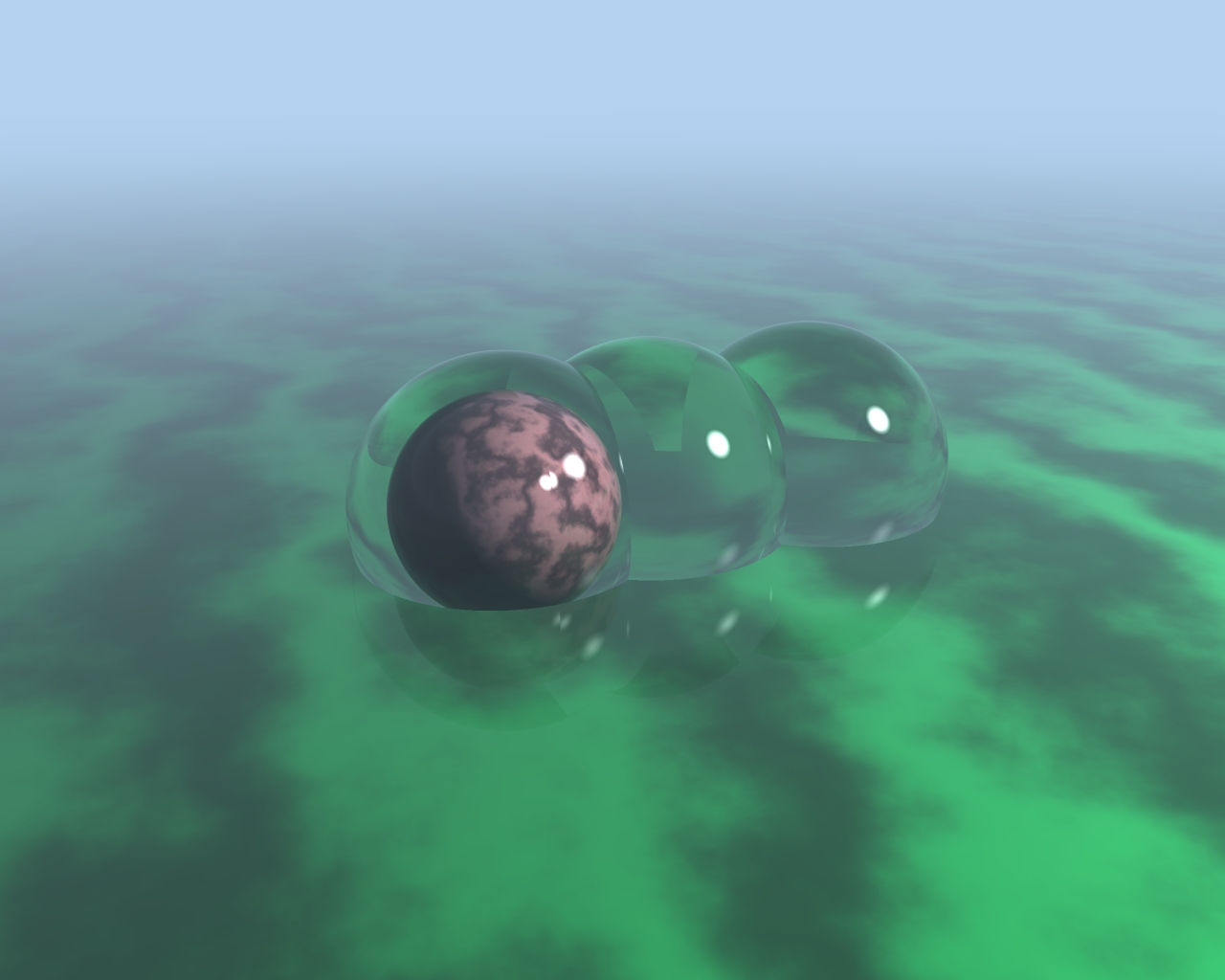
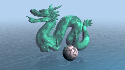
Refraction - Merged glass and attenuation
When I was playing with multiple glass objects I found out my raytracer had a problem. When two or more glass objects intersects some strange errors turns up on the faces inside the glass. To fix this I had to work out how to represents glass inside glass. This is the first test with multiple intersecting glass objects. Som bugs remains still and not all special cases can be traced correctly yet.

Click on image to enlarge
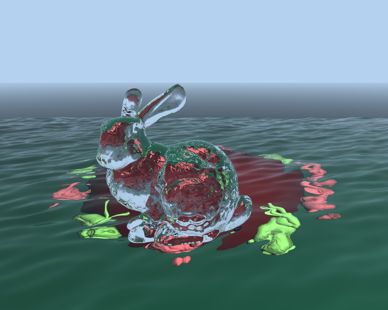
By figuring out how to represent surfaces better it turned out that it now was easy to add attenuation to transparent objects. The image below shows the effect of attenuating to a greenish color which appears like cryptonite.
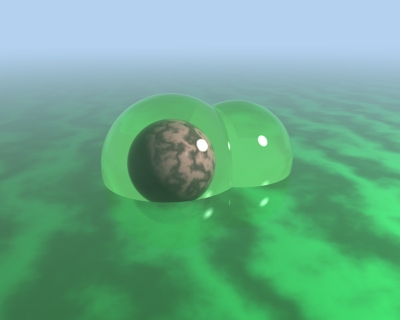
Click on image to enlarge
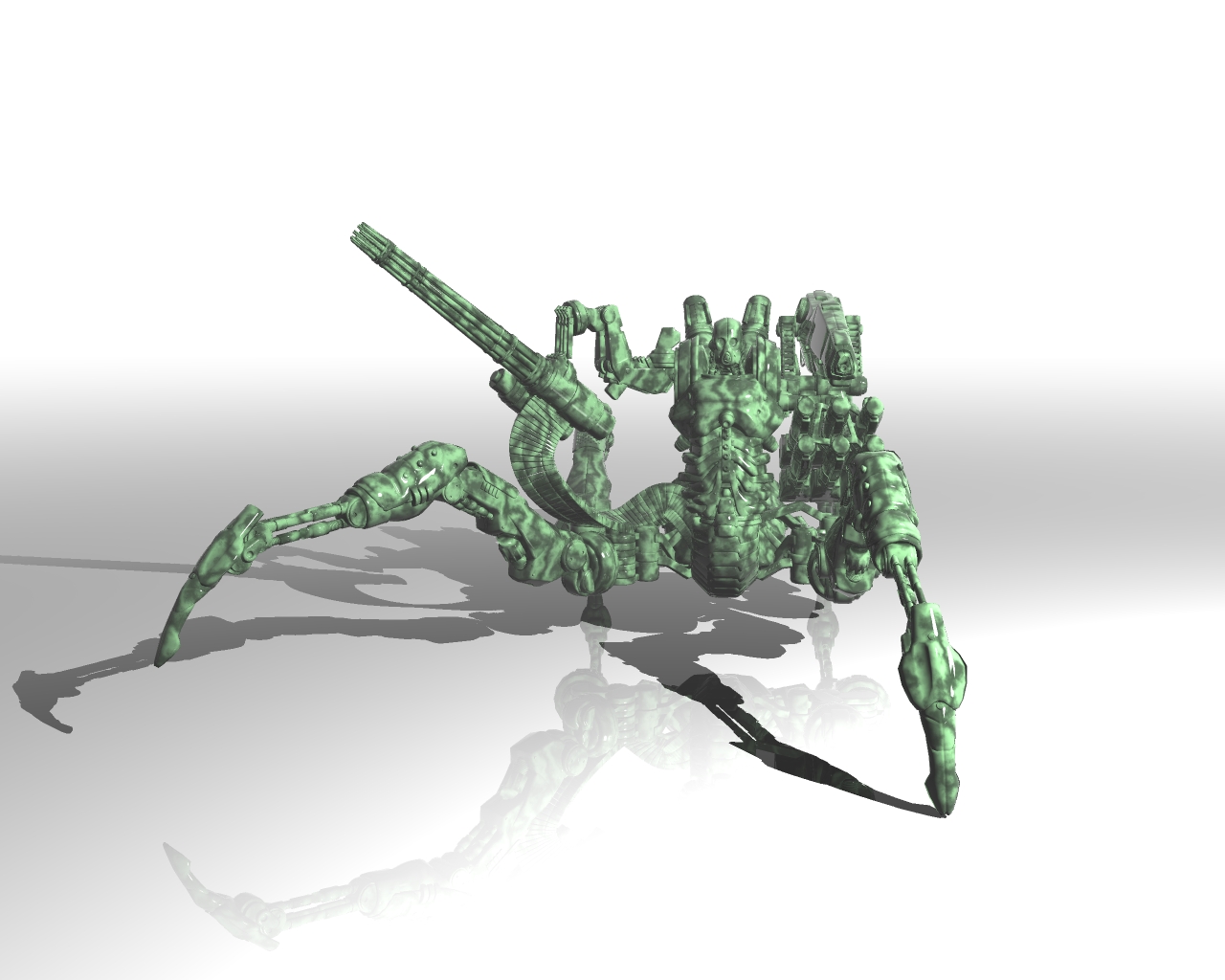
Xenotron - Mean model from Jonas Raagaard
The xenotron model below modelled by Jonas Raagaard really puts my raytracer to the test. Around 1 million triangles and a lot of details.
The model file was saved out to the .ASE format and I then made a simple converter from .ASE to my internal model format. The .ASE model file had a size of 148,464,558 bytes!
To see more work from Jonas and his original Xenotron image, try www.jonaz.dk

Click on image to enlarge
Bugs in Glass model
I found a bug in my glass model, that caused internal reflections to be calculated wrong. This is now fixed. Still the internal reflections needs some refactoring - more to come

Click on image to enlarge
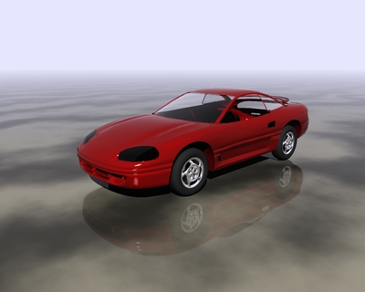
Mitsubishi and complex models
This is the first attempt of ray tracing more complex models. The model however lacks a few essential features such as seats and interior in general. Also my converter from .ASE to my gray model file format still does not handle scene structures, but only single meshes. So I had to export each part of the car (windows, hood, backhatch, wheels etc.) one at a time and then place it in my own scene description language.
I guess a better importer would be appropriate to implement now.
The car was rendered using my few supported materials, such as glass, plastic, diffuse and metal.
Click on image to enlarge
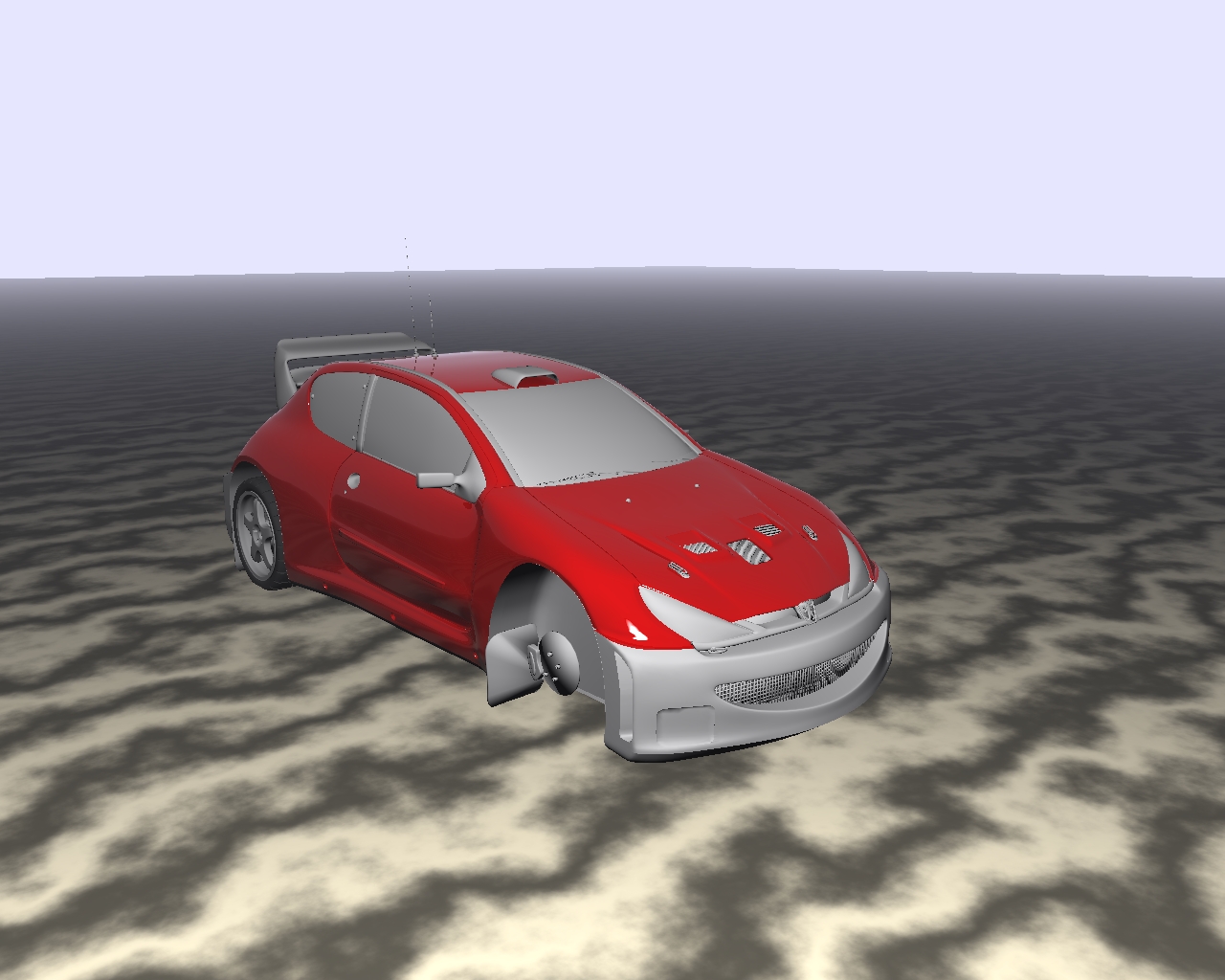
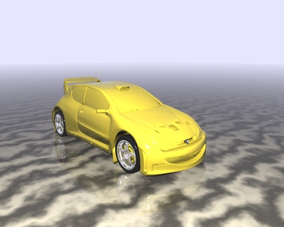
Peugeot206
A rather buggy image, because my new ASE to Grey converter is still not working optimal. I support multiple meshes now, but need to fix a few errors and include materials as well.

Click on image to enlarge
Found the missing wheel and tried out some other colors.
Click on image to enlarge
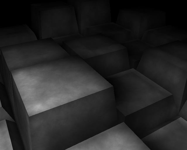
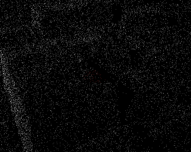
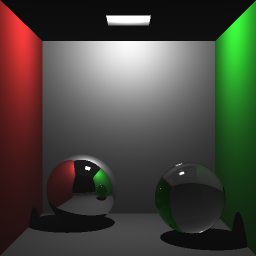
Photonmapping
So, finally, my first photon mapped image. I have implemented the photon emission, the photon-collection using a kd-tree and made a rough irradiance estimate for generating an image with soft shadows and global illumination

Click on image to enlarge
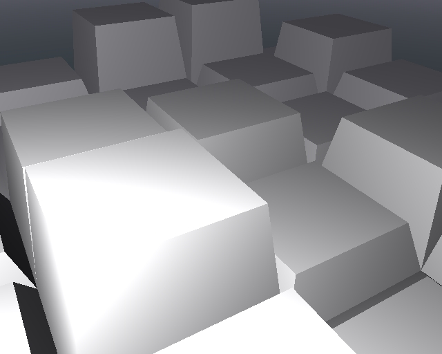
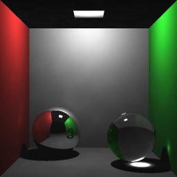
Same image using traditional ray tracing

Click on image to enlarge
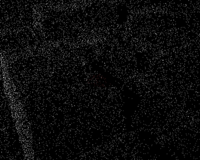
A view of the actual photon map
Click on image to enlarge
Caustics
After a long break, I've worked a bit more on photonmapping. This is a trial image featuring caustics.
|